Coursera - Supervised Machine Learning: Regression and Classification - Week 1 - Section 4 - Regression Model
2025年01月26日
Terminology


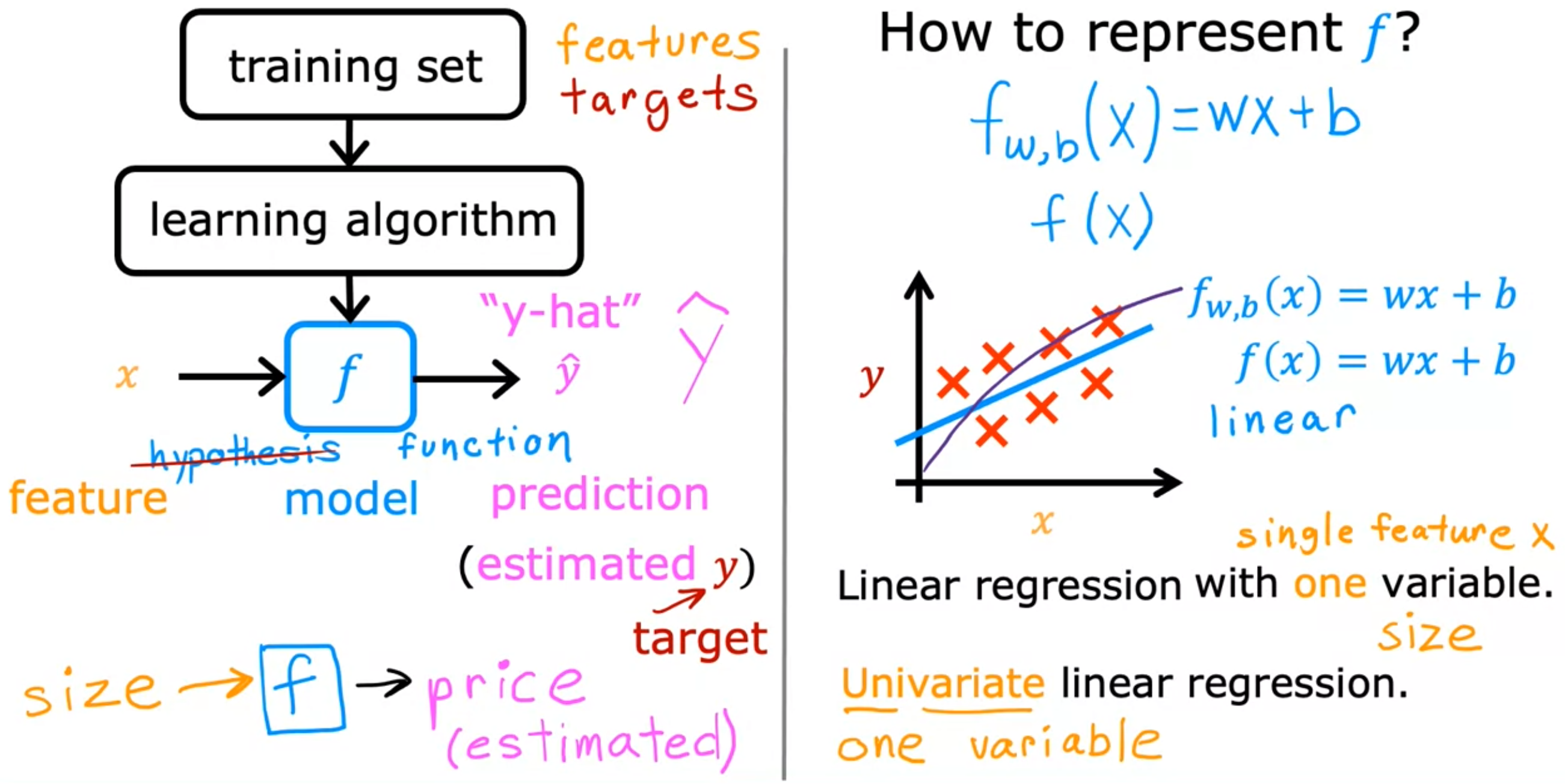
In machine learning, the convention is that y-hat is the estimate or the prediction for y.
The function f is called the model.
Another name for a linear model with one input variable is univariate linear regression, where uni means one in Latin, and where variate means variable. Univariate is just a fancy way of saying one variable.

For linear regression, the model is represented by \( f_{w, b}(x)=w x+b \). Which of the following is the output or "target" variable?
y is the true value for that training example, referred to as the output variable, or "target".
-
Training set


Eventually we're going to want to find values of w and b that make the cost function small.


The cost function used for linear regression is
\( J(w, b)=\frac{1}{2 m} \sum_{i=1}^m\left(f_{w, b}\left(x^{(i)}\right)-y^{(i)}\right)^2 \)
Which of these are the parameters of the model that can be adjusted?
w and b are parameters of the model, adjusted as the model learns from the data. They’re also referred to as "coefficients" or "weights".


When does the model fit the data relatively well, compared to other choices for parameter w?
When the cost is relatively small, closer to zero, it means the model fits the data better compared to other choices for w and b.


-


Week 1: Introduction to Machine Learning
Section 4: Regression Model
1. Video: Linear regression model part 1
Terminology

2. Video: Linear regression model part 2
In machine learning, the convention is that y-hat is the estimate or the prediction for y.
The function f is called the model.
Another name for a linear model with one input variable is univariate linear regression, where uni means one in Latin, and where variate means variable. Univariate is just a fancy way of saying one variable.

For linear regression, the model is represented by \( f_{w, b}(x)=w x+b \). Which of the following is the output or "target" variable?
- x
- \( \hat{y} \)
- m
- y
y is the true value for that training example, referred to as the output variable, or "target".
3. Lab: Optional lab: Model representation
--
4. Video: Cost function formula
Training set


Eventually we're going to want to find values of w and b that make the cost function small.


The cost function used for linear regression is
\( J(w, b)=\frac{1}{2 m} \sum_{i=1}^m\left(f_{w, b}\left(x^{(i)}\right)-y^{(i)}\right)^2 \)
Which of these are the parameters of the model that can be adjusted?
- w and b
- \( f_{w, b}\left(x^{(i)}\right) \)
- w only, because we should choose b=0
- \( \hat{y} \)
w and b are parameters of the model, adjusted as the model learns from the data. They’re also referred to as "coefficients" or "weights".
5. Video: Cost function intuition


When does the model fit the data relatively well, compared to other choices for parameter w?
- When w is close to zero.
- When the cost J is at or near a minimum.
- When fw(x) is at or near a minimum for all the values of x in the training set.
- When x is at or near a minimum.
When the cost is relatively small, closer to zero, it means the model fits the data better compared to other choices for w and b.
6. Video: Visualizing the cost function


-


7. Video: Visualization examples


